您现在的位置是：首页 >其他 >线性回归梯度下降法python实现网站首页其他

​
线性回归的公式：
$$h_{\theta }(x)={\theta }_0+{\theta }_1{x}_1+{\theta }_2{x}_2+\cdots +{\theta }_n{x}_n$$
其中，$h_{\theta }(x)$ 是预测值，$\theta$ 是模型参数，$x_1,x_2,\dots ,x_n$ 是输入特征。

梯度下降的更新公式：
$${\theta }_j={\theta }_j-\alpha \cdot \frac{1}{m}\sum _{i=1}^m\left(h_{\theta }(x^{(i)})-y^{(i)}\right)x_j^{(i)}$$
其中，${\theta }_j$ 是第 $j$ 个参数，$\alpha$ 是学习率，$m$ 是样本的数量，$h_{\theta }(x^{(i)})$ 是预测值，$y^{(i)}$ 是实际值，$x_j^{(i)}$ 是样本的第 $j$ 个特征。
线性回归的损失函数（均方误差）：

$$J(\theta )=\frac{1}{2m}\sum _{i=1}^m{\left(h_{\theta }(x^{(i)})-y^{(i)}\right)}^2$$

其中：

• $J(\theta )$ 是损失函数（成本函数），
• $m$ 是样本的数量，
• $h_{\theta }(x^{(i)})$ 是模型对第 $i$ 个样本的预测值，
• $y^{(i)}$ 是第 $i$ 个样本的实际值。

通常，在梯度下降中，我们通过最小化损失函数来优化模型参数 $\theta$。

import numpy as np
import matplotlib.pyplot as plt
import pandas as pd
def computeCost(X,y,theta):
    m = X.shape[0]
    part = np.power(((X@theta.T)-y),2)
    return np.sum(part)/(m*2)
def gradientDescent(X,y,theta,alpha,iterations):
    #副本
    temp = theta
    #样本数量
    m = X.shape[0]
    #特征数
    params = theta.shape[1]
    #记录每一次的成本变化
    costs = np.zeros(iterations)
    #迭代iterations次
    for i in range(iterations):
        error = X@theta.T-y
        for j in range(params):
            temp[0,j] = temp[0,j] - (alpha/m)*np.sum(np.multiply(error,X[:,j:j+1]))
        theta = temp
        costs[i] = computeCost(X,y,theta)
    return theta, costs
# 读取数据，dataframe
data = pd.read_csv('ex1data1.txt', header=None,names = ["population","profits"])
#插入一行1，作为线性回归函数的常数项
data.insert(0,"Ones",1)
print(data.head())
cols = data.shape[1]
#切片第二项也要用:，保持是dataframe
X = data.iloc[:,0:cols-1]
y = data.iloc[:,cols-1:cols]
#theta都初始化为0，np.array默认是行向量
theta = np.zeros((1,cols-1))
#将dataframe转化为np.array
X = X.to_numpy()
y = y.to_numpy()
print(X.shape)
print(y.shape)
print(theta.shape)
alpha = 0.01
iterations = 1000
theta, costs =gradientDescent(X,y,theta,alpha,iterations)
print(costs[iterations-1])
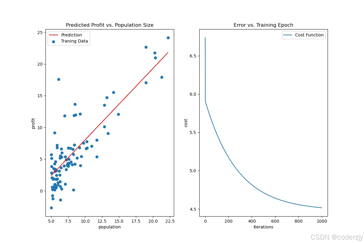
x = np.linspace(data.population.min(), data.population.max(),100)
f = theta[0,0] + theta[0,1] * x
fig = plt.figure()
#fig 为整个画图区域，ax为子图的集合
#当nrows=1或ncols=1时为一维数组，此时下标索引只有一个维度，否则是两个维度
fig,ax = plt.subplots(figsize=(12,8),nrows=1,ncols=2)
ax[0].plot(x, f, 'r', label='Prediction')
ax[0].set_title('Predicted Profit vs. Population Size')
ax[0].set_xlabel('population')
ax[0].set_ylabel('profit')
ax[0].scatter(data.population, data.profits, label='Traning Data')
ax[0].legend()
#np.arange(iterations) 的意思是 生成从 0 到 iterations-1 的整数数组。
#np.arange(start, stop, step, dtype) 用于生成等间隔的数组
ax[1].plot(np.arange(iterations),costs,label='Cost Function')
ax[1].set_title('Error vs. Training Epoch')
ax[1].set_xlabel('iterations')
ax[1].set_ylabel('cost')
ax[1].legend()
plt.show()