您现在的位置是:首页 >技术杂谈 >第P1周:Pytorch实现mnist手写数字识别网站首页技术杂谈
第P1周:Pytorch实现mnist手写数字识别
简介第P1周:Pytorch实现mnist手写数字识别
- **🍨 本文为[🔗365天深度学习训练营](https://mp.weixin.qq.com/s/rnFa-IeY93EpjVu0yzzjkw) 中的学习记录博客**
- **🍖 原作者:[K同学啊](https://mtyjkh.blog.csdn.net/)**
语言环境:Python 3.9
开发工具: Jupyter Lab
深度学习环境:pytorch
import torch
import torch.nn as nn
import matplotlib.pyplot as plt
import torchvision
第一步:导入库
- torch:PyTorch的核心库,用于张量操作和深度学习模型的实现。
- torch.nn:提供构建神经网络的工具。
- matplotlib.pyplot:用于绘制图形,主要用于结果的可视化。
- torchvision:包含了常用的数据集和图像处理工具,这里用来加载MNIST数据集
device torch.device("cuda" if torch.cuda.is_available() else "cpu")
device
第二步:设置计算设备
这行代码检测是否有CUDA(即GPU)可用。如果GPU可用,则将设备设置为GPU;如果没有,则使用CPU
train_ds = torchvision.datasets.MNIST('data',
                                      train=True,
                                      transform=torchvision.transforms.ToTensor(), # 将数据类型转化为Tensor
                                      download=True)

test_ds  = torchvision.datasets.MNIST('data',
                                      train=False,
                                      transform=torchvision.transforms.ToTensor(), # 将数据类型转化为Tensor
                                      download=True)
第三步:加载数据集
- train_ds:加载MNIST训练数据集并将图像转换为张量。
- test_ds:加载MNIST测试数据集,处理方式相同。
- transform=torchvision.transforms.ToTensor():将图像数据转换为张量格式
batch_size = 32
train_dl = torch.utils.data.DataLoader(train_ds, batch_size=batch_size, shuffle=True)
test_dl  = torch.utils.data.DataLoader(test_ds, batch_size=batch_size)
torch.Size([32, 1, 28, 28])
第四步:DataLoader设置
- DataLoader:将数据集包装成可迭代的数据加载器,方便按批次加载和打乱数据。
- batch_size:每个批次的数据量,设置为32。
- shuffle=True:在训练时打乱数据顺序,避免数据顺序影响训练结果
plt.figure(figsize=(20, 5))
for i, imgs in enumerate(imgs[:20]):
    npimg = np.squeeze(imgs.numpy())
    plt.subplot(2, 10, i+1)
    plt.imshow(npimg, cmap=plt.cm.binary)
    plt.axis('off')
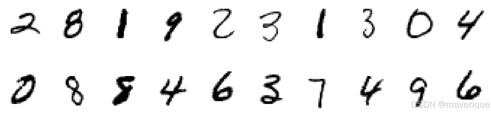
第五步:可视化部分数据
这段代码将训练数据集中的前20张图像可视化,显示在一个2行10列的网格中
class Model(nn.Module):
    def __init__(self):
        super().__init__()
        self.conv1 = nn.Conv2d(1, 32, kernel_size=3)  # 第一层卷积,卷积核大小为3x3
        self.pool1 = nn.MaxPool2d(2)                  # 设置池化层,池化核大小为2x2
        self.conv2 = nn.Conv2d(32, 64, kernel_size=3) # 第二层卷积,卷积核大小为3x3
        self.pool2 = nn.MaxPool2d(2)
        self.fc1 = nn.Linear(1600, 64)                # 全连接层
        self.fc2 = nn.Linear(64, num_classes)         # 输出层
第六步:定义神经网络模型
这里定义了一个卷积神经网络(CNN)模型:
- Conv2d:卷积层,用于提取特征。
- MaxPool2d:池化层,用于下采样,减少图像的空间尺寸。
- Linear:全连接层,用于分类。
def forward(self, x):
    x = self.pool1(F.relu(self.conv1(x)))
    x = self.pool2(F.relu(self.conv2(x)))
    x = torch.flatten(x, start_dim=1)
    x = F.relu(self.fc1(x))
    x = self.fc2(x)
    return x
第七步:前向传播
这段代码定义了前向传播过程:
- 每一层卷积后,应用ReLU激活函数和池化操作。
- 将卷积后的数据展平(flatten),然后传递给全连接层
from torchinfo import summary
model = Model().to(device)
summary(model)
=================================================================
Layer (type:depth-idx)                   Param #
=================================================================
Model                                    --
├─Conv2d: 1-1                            320
├─MaxPool2d: 1-2                         --
├─Conv2d: 1-3                            18,496
├─MaxPool2d: 1-4                         --
├─Linear: 1-5                            102,464
├─Linear: 1-6                            650
=================================================================
Total params: 121,930
Trainable params: 121,930
Non-trainable params: 0
=================================================================
第八步:打印模型
summary(model) 打印模型的结构概况,包括每层的参数数量和输出尺寸
loss_fn = nn.CrossEntropyLoss()
learn_rate = 1e-2
opt = torch.optim.SGD(model.parameters(), lr=learn_rate)
第九步:损失函数和优化器
- CrossEntropyLoss:交叉熵损失函数,常用于分类任务。
- SGD (随机梯度下降):用于优化模型,调整权重以最小化损失
def train(dataloader, model, loss_fn, optimizer):
    train_loss, train_acc = 0, 0
    for X, y in dataloader:
        X, y = X.to(device), y.to(device)
        pred = model(X)
        loss = loss_fn(pred, y)
        optimizer.zero_grad()
        loss.backward()
        optimizer.step()
        train_acc += (pred.argmax(1) == y).type(torch.float).sum().item()
        train_loss += loss.item()
    return train_acc / size, train_loss / num_batches
第十步:训练循环
- 对每个批次的数据进行前向传播,计算损失。
- 进行反向传播,更新模型参数。
- 计算训练集的损失和准确率。
def test(dataloader, model, loss_fn):
    with torch.no_grad():
        for imgs, target in dataloader:
            imgs, target = imgs.to(device), target.to(device)
            target_pred = model(imgs)
            loss = loss_fn(target_pred, target)
            test_loss += loss.item()
            test_acc += (target_pred.argmax(1) == target).type(torch.float).sum().item()
    return test_acc / size, test_loss / num_batches
第十一步 :测试循环
epochs = 5
train_loss = []
train_acc = []
test_loss = []
test_acc = []

for epoch in range(epochs):
    model.train()
    epoch_train_acc, epoch_train_loss = train(train_dl, model, loss_fn, opt)
    model.eval()
    epoch_test_acc, epoch_test_loss = test(test_dl, model, loss_fn)
    train_acc.append(epoch_train_acc)
    train_loss.append(epoch_train_loss)
    test_acc.append(epoch_test_acc)
    test_loss.append(epoch_test_loss)
Epoch: 1, Train_acc:99.3%, Train_loss:0.022, Test_acc:98.8%,Test_loss:0.036
Epoch: 2, Train_acc:99.4%, Train_loss:0.021, Test_acc:98.8%,Test_loss:0.034
Epoch: 3, Train_acc:99.4%, Train_loss:0.021, Test_acc:98.9%,Test_loss:0.033
Epoch: 4, Train_acc:99.4%, Train_loss:0.019, Test_acc:98.8%,Test_loss:0.036
Epoch: 5, Train_acc:99.4%, Train_loss:0.018, Test_acc:98.9%,Test_loss:0.033
Done
第十二步:训练模型
模型训练5个周期,每个周期分别训练和测试:
- 记录每个周期的训练和测试的损失和准确率
plt.figure(figsize=(12, 3))
plt.subplot(1, 2, 1)
plt.plot(epochs_range, train_acc, label='Training Accuracy')
plt.plot(epochs_range, test_acc, label='Test Accuracy')
plt.legend(loc='lower right')
plt.title('Training and Validation Accuracy')

plt.subplot(1, 2, 2)
plt.plot(epochs_range, train_loss, label='Training Loss')
plt.plot(epochs_range, test_loss, label='Test Loss')
plt.legend(loc='upper right')
plt.title('Training and Validation Loss')
plt.show()
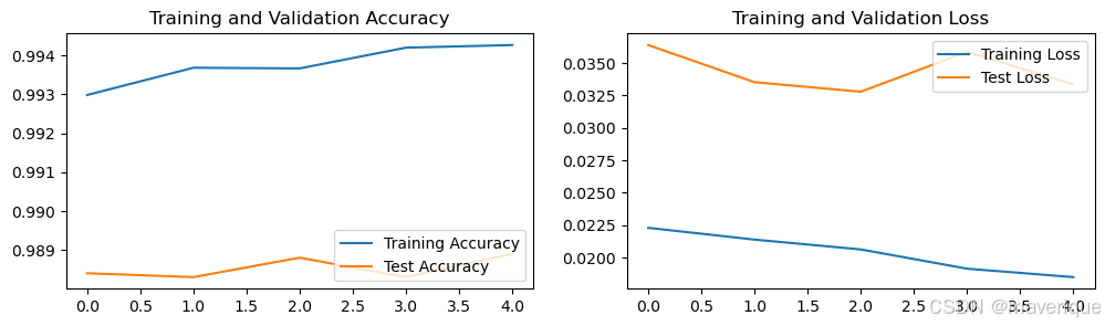
风语者!平时喜欢研究各种技术,目前在从事后端开发工作,热爱生活、热爱工作。




站长推荐
- QT多线程的5种用法,通过使用线程解决UI主界面的耗时操作代码,防止界面卡死。
 QT多线程的5种用法,通过使用线程解决UI主界面的耗时操作代码,防止界面卡死。...
 - U8W/U8W-Mini使用与常见问题解决
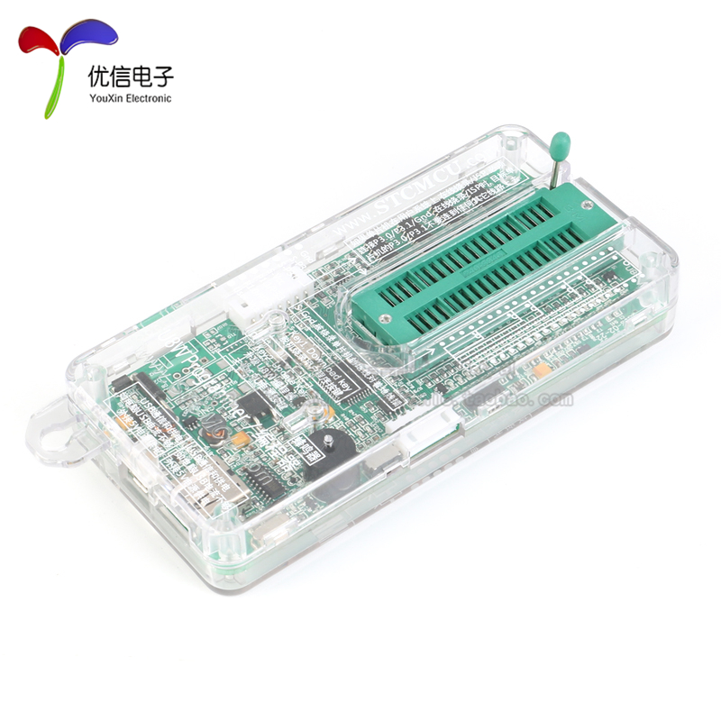 U8W/U8W-Mini使用与常见问题解决
 - stm32使用HAL库配置串口中断收发数据(保姆级教程)
 stm32使用HAL库配置串口中断收发数据(保姆级教程)
 - 分享几个国内免费的ChatGPT镜像网址(亲测有效)
 分享几个国内免费的ChatGPT镜像网址(亲测有效)
 - Allegro16.6差分等长设置及走线总结
 Allegro16.6差分等长设置及走线总结