您现在的位置是:首页 >技术交流 >[AI学习] 一元线性回归网站首页技术交流
[AI学习] 一元线性回归
一元线性回归
介绍
线性回归(Linear Regression)是一种用于建模和预测变量之间线性关系的统计方法。它假设因变量(目标变量)与一个或多个自变量(特征变量)之间存在线性关系,并通过拟合最佳直线(或超平面)来描述这种关系。
核心概念
1.模型形式
一元线性回归: 只有一个自变量,形式为:
y
=
w
1
x
+
b
y=w_1x+b
y=w1x+b
其中,y是因变量,x是自变量,w1是权重(系数),b是截距
多元线性回归:包含包含多个自变量,形式为:
y
=
w
1
x
1
+
w
2
x
2
+
⋯
+
w
n
x
n
+
b
y=w_1x_1+w_2x_2+⋯+w_nx_n+b
y=w1x1+w2x2+⋯+wnxn+b
其中,
x
1
,
x
2
,
…
,
x
n
x_1,x_2,…,x_n
x1,x2,…,xn是多个自变量,
w
1
,
w
2
,
…
,
w
n
w_1,w_2,…,w_n
w1,w2,…,wn是对应的权重。
2. 目标
找到一组权重 ( w 1 , w 2 , … , w n ) (w_1,w_2,…,w_n) (w1,w2,…,wn)和截距(b),使得模型的预测值和真实值之间的误差最小
3. 损失函数
用于衡量预测值与真实值的差距:
均方误差(Mean Squared Error, MSE)
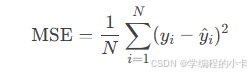
其中
y
i
是真实值
y
^
是预测值,
N
是样本数量
其中 y_i 是真实值hat{y}是预测值,N是样本数量
其中yi是真实值y^是预测值,N是样本数量,
4.代价函数
是所有样本误差的平均,也就是损失函数的平均。
5.参数估计
-
梯度下降:通过迭代优化算法逐步调整参数,最小化损失函数。 梯度下降算法(我之前的另一篇)
-
最小二乘法:通过数学推导直接求实例:
假设用面积(x)预测房价(y),模型可能拟合出:
y = 1.2 x + 40 y=1.2x+40 y=1.2x+40
表示每增加1平方米,房价增加1.2万元,基础房价(截距)为40万元。解权重和截距的闭式解。
优缺点:
- 优点:简单、可解释性强、计算高效。
- 缺点:对非线性关系或复杂数据模式拟合能力有限,易受异常值影响
数据集和特征
数据集
定义:数据集是用于训练或测试模型的结构化数据集合,通常以表格形式组织(如 CSV、Excel 文件或数据库表)。每一行代表一个样本(Sample),每一列代表一个属性(即特征或变量)。
数据集的组成
● 样本(Samples):数据集中每一行是一个独立的观测值(如一个用户、一件商品、一条记录)。
● 特征(Features):每一列是描述样本的某个属性(如年龄、温度、像素值等)。
● 标签/目标变量(Label/Target)(监督学习中):需要预测的变量(如房价、分类结果)。
示例
| 面积(平方米) | 房间数 | 楼层 | 房价(万元) |
|---|---|---|---|
| 80 | 2 | 5 | 100 |
| 120 | 3 | 10 | 250 |
| 60 | 1 | 2 | 70 |
- 样本数:3 条(3 行)
- 特征:面积、房间数、楼层
- 标签:房价(目标变量)
数据集的类型
- 结构化数据:表格形式,适合传统机器学习(如房价预测)。
- 非结构化数据:图像、文本、音频等,需转换为特征(如像素、词向量)后使用。
- 时间序列数据:按时间顺序排列(如股票价格、传感器数据)。
特征
定义:特征是描述样本的属性或变量,是模型的输入(自变量)。特征的质量直接影响模型性能。
特征的类型
- 数值型特征(Numerical Features)
○ 连续型:可无限细分(如温度、体重)。
○ 离散型:取整数值(如房间数、点击次数)。 - 类别型特征(Categorical Features)
○ 有序类别:有顺序关系(如评分:高、中、低)。
○ 无序类别:无顺序关系(如颜色、城市名)。 - 文本特征:需转换为数值(如词频、TF-IDF)。
- 时间特征:日期、时间戳(需分解为年、月、日等)。
应用
- 房价预测:
○*特征:面积,地段
○ 标签:房价 - 用户流失预测:
○ 特征:登录频率,使用实操
○ 标签: 是否流失
代码实例
以下代码采用的 python 进行编写
首先需要准备一下数据集
这里我采用的是 kaggle 上面下载的一组数据集,为工作年限与薪资的数据集
https://www.kaggle.com/datasets/abhishek14398/salary-dataset-simple-linear-regression?resource=download
部分数据如下
,YearsExperience,Salary
0,1.2000000000000002,39344.0
1,1.4000000000000001,46206.0
2,1.6,37732.0
3,2.1,43526.0
...
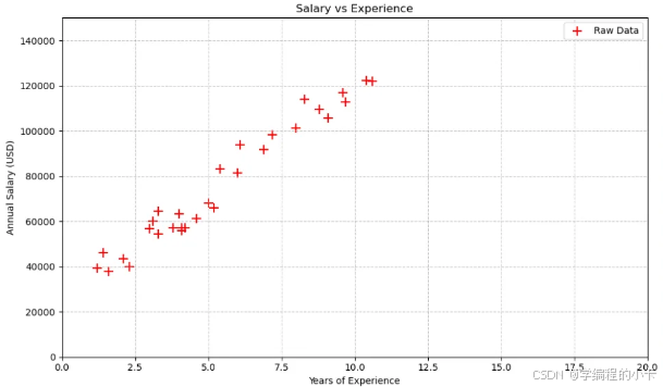
数据图
基于这组数据绘制一下图
import matplotlib.pyplot as plt  # 数据可视化
import numpy as np  # 数值计算
import pandas as pd  # 数据处理

salary_df = pd.read_csv("./Salary_dataset.csv")  # 使用pd.read_csv更规范的写法

# 获取数据集维度信息
num_samples, num_features = salary_df.shape
print(f"样本数量: {num_samples}, 特征数量: {num_features}")  # 使用f-string格式化

# 提取特征和标签(直接使用DataFrame列访问更高效)
years_exp = salary_df['YearsExperience'].tolist()  # 工作经验作为特征
salary = salary_df['Salary'].tolist()             # 薪资作为标签

# 创建画布和坐标系
fig = plt.figure(figsize=(10, 6))  # 设置画布尺寸
ax = fig.add_subplot(111)          # 创建子图

# 设置坐标系参数
ax.set(
    xlim=[0, 20],                  # X轴范围(工作年限)
    ylim=[0, 150000],              # Y轴范围(薪资)
    title='Salary vs Experience',  # 图表标题
    xlabel='Years of Experience',  # X轴标签
    ylabel='Annual Salary (USD)'   # Y轴标签
)

# 绘制散点图
ax.scatter(
    years_exp,
    salary,
    color='red',
    marker='+',
    s=100,           # 标记大小
    label='Raw Data' # 图例标签
)

# 添加网格线
ax.grid(True, linestyle='--', alpha=0.7)

# 显示图表
plt.legend()
plt.tight_layout()  # 自动调整布局
plt.show()
于该数据建立一元线性回归模型
y
=
w
1
+
x
y = w_1 + x
y=w1+x
我们可以等价与
h
θ
(
x
)
=
θ
0
+
θ
1
h_θ(x) = θ_0 + θ_1
hθ(x)=θ0+θ1
代价函数
均方误差(MSE)的代价函数为:
J
(
θ
0
,
θ
1
)
=
1
2
m
∑
i
=
1
m
(
h
θ
(
x
(
i
)
)
−
y
(
i
)
)
2
J( heta_0, heta_1) = frac{1}{2m} sum_{i=1}^{m} (h_ heta(x^{(i)}) - y^{(i)})^2
J(θ0,θ1)=2m1i=1∑m(hθ(x(i))−y(i))2
补充:这里采用 1 / 2 是为了梯度下降的时候简化计算
偏导数
对于
θ
0
和
θ
1
求偏导
对于 θ_0 和 θ_1求偏导
对于θ0和θ1求偏导
对
θ
0
:
对 θ_0:
对θ0:
∂
J
∂
θ
0
=
1
m
∑
i
=
1
m
(
h
θ
(
x
(
i
)
)
−
y
(
i
)
)
frac{partial J}{partial heta_0} = frac{1}{m} sum_{i=1}^{m} (h_ heta(x^{(i)}) - y^{(i)})
∂θ0∂J=m1i=1∑m(hθ(x(i))−y(i))
对
θ
1
:
对 θ_1:
对θ1:
∂
J
∂
θ
1
=
1
m
∑
i
=
1
m
(
h
θ
(
x
(
i
)
)
−
y
(
i
)
)
x
(
i
)
frac{partial J}{partial heta_1} = frac{1}{m} sum_{i=1}^{m} (h_ heta(x^{(i)}) - y^{(i)})x^{(i)}
∂θ1∂J=m1i=1∑m(hθ(x(i))−y(i))x(i)
对应代码 :
theta0
def compute_gradient_theta0(x: np.ndarray, y: np.ndarray,
                            theta0: float, theta1: float) -> float:
    """计算代价函数关于theta0的偏导数
    Args:
        x: 特征向量(工作年限)
        y: 目标向量(薪资)
        theta0: 当前截距参数
        theta1: 当前斜率参数
    Returns:
        float: theta0的梯度值
    """
    m = len(x)
    hypothesis = theta0 + theta1 * x
    return np.sum(hypothesis - y) / m  # 向量化计算
theta1
def compute_gradient_theta1(x: np.ndarray, y: np.ndarray,
                            theta0: float, theta1: float) -> float:
    """计算代价函数关于theta1的偏导数"""
    m = len(x)
    hypothesis = theta0 + theta1 * x
    return np.sum((hypothesis - y) * x) / m  # 向量化计算
代价函数
def compute_cost(x: np.ndarray, y: np.ndarray,
                 theta0: float, theta1: float) -> float:
    """计算均方误差代价函数"""
    m = len(x)
    hypothesis = theta0 + theta1 * x
    return np.sum((hypothesis - y) ** 2) / (2 * m)
梯度下降
def gradient_descent(x: np.ndarray, y: np.ndarray,
                     alpha: float, iterations: int) -> tuple:
    """执行梯度下降算法
    Args:
        alpha: 学习率
        iterations: 迭代次数
    Returns:
        tuple: (最优theta0, 最优theta1)
    """
    theta0, theta1 = 0.0, 0.0
    cost_history = []  # 记录代价变化

    for i in range(1, iterations + 1):
        grad0 = compute_gradient_theta0(x, y, theta0, theta1)
        grad1 = compute_gradient_theta1(x, y, theta0, theta1)

        theta0 -= alpha * grad0
        theta1 -= alpha * grad1

        # 每1000次记录代价(可选)
        if i % 1000 == 0:
            cost = compute_cost(x, y, theta0, theta1)
            cost_history.append(cost)

    return theta0, theta1
全部代码
import matplotlib.pyplot as plt
import numpy as np
import pandas as pd # 使用标准别名
# --------------------------
# 核心算法函数
# --------------------------
def compute_gradient_theta0(x: np.ndarray, y: np.ndarray,
theta0: float, theta1: float) -> float:
"""计算代价函数关于theta0的偏导数
Args:
x: 特征向量(工作年限)
y: 目标向量(薪资)
theta0: 当前截距参数
theta1: 当前斜率参数
Returns:
float: theta0的梯度值
"""
m = len(x)
hypothesis = theta0 + theta1 * x
return np.sum(hypothesis - y) / m # 向量化计算
def compute_gradient_theta1(x: np.ndarray, y: np.ndarray,
theta0: float, theta1: float) -> float:
"""计算代价函数关于theta1的偏导数"""
m = len(x)
hypothesis = theta0 + theta1 * x
return np.sum((hypothesis - y) * x) / m # 向量化计算
def compute_cost(x: np.ndarray, y: np.ndarray,
theta0: float, theta1: float) -> float:
"""计算均方误差代价函数"""
m = len(x)
hypothesis = theta0 + theta1 * x
return np.sum((hypothesis - y) ** 2) / (2 * m)
def gradient_descent(x: np.ndarray, y: np.ndarray,
alpha: float, iterations: int) -> tuple:
"""执行梯度下降算法
Args:
alpha: 学习率
iterations: 迭代次数
Returns:
tuple: (最优theta0, 最优theta1)
"""
theta0, theta1 = 0.0, 0.0
cost_history = [] # 记录代价变化
for i in range(1, iterations + 1):
grad0 = compute_gradient_theta0(x, y, theta0, theta1)
grad1 = compute_gradient_theta1(x, y, theta0, theta1)
theta0 -= alpha * grad0
theta1 -= alpha * grad1
# 每1000次记录代价(可选)
if i % 1000 == 0:
cost = compute_cost(x, y, theta0, theta1)
cost_history.append(cost)
return theta0, theta1
# --------------------------
# 主程序
# --------------------------
def main():
# 数据准备
data = pd.read_csv('./Salary_dataset.csv')
x = data['YearsExperience'].values # 转换为numpy数组
y = data['Salary'].values
# 超参数设置
alpha = 0.01 # 学习率
n = 5000
# 执行梯度下降
theta0, theta1 = gradient_descent(x, y, alpha, n)
# 结果输出
final_cost = compute_cost(x, y, theta0, theta1)
print(f"经过 {n} 次迭代:")
print(f"最终代价值: {final_cost:.2f}")
print(f"最优参数:theta0 = {theta0:.2f}, theta1 = {theta1:.2f}")
# 预测示例
# 注意:20年经验超出数据集范围,预测结果可能不可靠
experience_years = [4, 20]
for years in experience_years:
prediction = theta0 + theta1 * years
print(f"预测 {years} 年工作经验薪资: ${prediction:,.2f}")
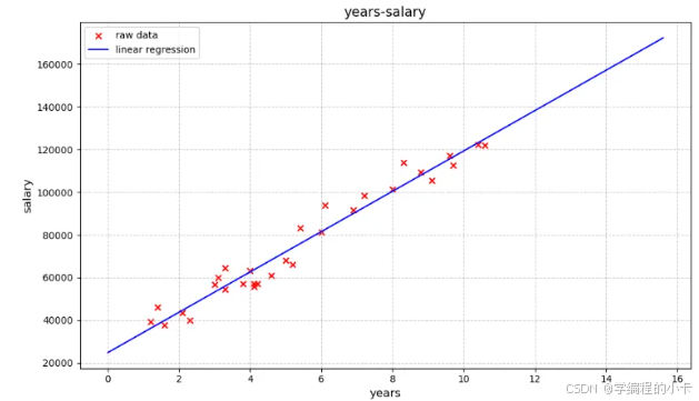
# 可视化
plt.figure(figsize=(10, 6))
plt.scatter(x, y, color='red', marker='x', label='raw data')
# 生成回归线(扩展到数据范围外)
x_vals = np.linspace(0, x.max() + 5, 100)
y_vals = theta0 + theta1 * x_vals
plt.plot(x_vals, y_vals, 'b-', label='linear regression')
plt.title('years-salary', fontsize=14)
plt.xlabel('years', fontsize=12)
plt.ylabel('salary', fontsize=12)
plt.legend()
plt.grid(linestyle='--', alpha=0.7)
plt.tight_layout()
plt.show()
if __name__ == '__main__':
main()


站长推荐
- U8W/U8W-Mini使用与常见问题解决
 U8W/U8W-Mini使用与常见问题解决
 - QT多线程的5种用法,通过使用线程解决UI主界面的耗时操作代码,防止界面卡死。
 QT多线程的5种用法,通过使用线程解决UI主界面的耗时操作代码,防止界面卡死。...
 - stm32使用HAL库配置串口中断收发数据(保姆级教程)
 stm32使用HAL库配置串口中断收发数据(保姆级教程)
 - 分享几个国内免费的ChatGPT镜像网址(亲测有效)
 分享几个国内免费的ChatGPT镜像网址(亲测有效)
 - SpringSecurity实现前后端分离认证授权
 SpringSecurity实现前后端分离认证授权