您现在的位置是：首页 >其他 >Deep Learning for 3D Point Clouds: A Survey网站首页其他

Guo Y, Wang H, Hu Q, et al. Deep learning for 3d point clouds: A survey[J]. IEEE Transactions on Pattern Analysis and Machine Intelligence, 2020.
之前组会要分享的一篇综述，太长了没读完，不知道啥时候能写完。。

一、摘要

最近，点云学习因其在计算机视觉、自动驾驶和机器人等许多领域的广泛应用而引起越来越多的关注。作为人工智能领域的主导技术，深度学习已成功用于解决各种二维视觉问题。然而，由于使用深度神经网络处理点云所面临的独特挑战，点云上的深度学习仍处于起步阶段。最近，点云上的深度学习甚至变得蓬勃发展，人们提出了许多方法来解决这一领域的不同问题。为了促进未来的研究，本文全面回顾了点云深度学习方法的最新进展。

本文综述了三维理解的最新方法，包括三维形状分类、三维目标检测与跟踪、三维场景与目标分割。对这些方法进行了全面的分类和性能比较。文中还介绍了各种方法的优缺点，并列举了潜在的研究方向。
三维数据在不同领域有着广泛的应用，包括自动驾驶、机器人、遥感技术和医疗。

一些公开数据集：ModelNet、ShapeNet、ScanObjectNN、PartNet、S3DIS、ScanNet、Semantic3D、ApolloCar3D、the KITTI Vision Benchmark Suite 。这些公开的数据集促进了三维点云深度学习的研究，越来越多的方法被提出来解决与点云相关的各种问题，包括三维形状分类、三维目标检测与跟踪、三维点云分割、三维点云配准、六自由度姿态估计和三维重建等。

二、背景

三、 3D shape classification

1. Multi-view based : project an unstructured point cloud into 2D images.【基于多视：将非结构化的点云投影到二维图像中。】
2. Volumetric-based: convert a point cloud into a 3D volumetric representation. well-established 2D or 3D convolutional networks are leveraged to achieve shape classification.【基于体积：将点云转换为三维体积表示。利用成熟的二维或三维卷积网络来实现形状分类。】
3. Point-based: do not introduce explicit information loss.【基于点：不引入明确的信息损失】
   

3.1 Multi-view based Methods(project 3D shape into multi-views and extract view-wise features)【多视】

1. MVCNN: max-pooling, only retains maximum elements.【采用最大池化，仅保留最大特征】
2. MHBN: integrate local conv features by bilinear pooling -> compact global descriptor.【通过双线性池化整合局部的卷积特征】
3. a relation network to exploit inter-relationship over a group views -> discriminative 3D object representation.
4. View-GCN: multi views as graph nodes. Core layer composing of local graph convolution. Graph apply non-local message passing and selective view-sampling.【将“多视”视为图节点，核心层由局部图卷积组成。应用非局部的信息传递和选择性的视图采样。】

3.2 Volumetric-based Methods(point cloud => 3D grids)【3D点云->3D网格】

1. VoxNet: volumetric occupancy network to achieve robust 3D object recognition.【volumetric occupancy网络来实现强大的三维物体识别。】

2. 3D ShapeNets: conv deep belief-based network to learn distributions of points from various 3D shapes.【基于信念的深度网络学习各种三维形状的点的分布情况。】

3. OctNet: 1st hierarchically partition point cloud using a hybrid grid-octree structure.
   Represent the scene with several shallow octrees along a regular grid.

4. Octree-based CNN: The average normal vectors(法向量) are fed into the network, and 3D CNN is applied on the octants. 【八叉树】

   OctNet requires much less memory and runtime for high-resolution point clouds.【对于高分辨率的点云，八叉树需要更少的内存并且更快。】

5. PointGrid: Integrate point and grid represent for efficient point cloud processing. Use 3D Conv to extract features by sampling from each embedding volumetric grid cell.【 整合点和网格来实现高效的点云处理。使用3D Conv从每个嵌入的体积网格单元取样来提取特征。】

6. Ben-Shabat: input point cloud -> 3D grids -> 3D modified Fisher Vector (3DmFV). Use CNN learn global representation.【point cloud -> 3D grids -> 3D modified Fisher Vector 】

3.3 Point-based Methods

Depending the network architecture used for the feature learning of each point.

3.3.1 Pointwise MLP Methods

Pointwise MLP Methods model each point independently with several shared Multi-Layer Perceptrons (MLPs) and then aggregate a global feature using a symmetric aggregation function.

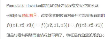
1. PointNet: take point cloud as input achieve permutation invariance using a symmetric function. (ad: Typical deep learning methods for 2D images cannot be directly applied to 3D point clouds due to their inherent data irregularities)
   
   

2. Deep Sets: achieve permutation invariance by summing all representations up and applying nonlinear transformations.

3. PointNet++: (features learned independently from each point, the local structure between points is ignored.) its hierarchy is composed of 3 layers: the sampling layer, the grouping layer, the PointNet based learning layer. Learn features from local geometric structure and layer by layer.

4. MoNet: similar to PointNet, but take a finite set of moments as input.

5. Point Attention Transformers: (a. represent each point by its own position and neighbor’s relative positions. (b. learn high dimensional features by MLPs.

6. Group Shuffle Attention: capture relations between points. Use a permutation invariance, differentiable and trainable end2end Gumbel Subset Sampling (GSS) layer to learn hierarchy features.

7. PointWeb: improve point features from context of local neighborhood using Adaptive Feature Adjustment (AFA).

8. Structural Relational Network: learn structural relational features between local structures using MLPs.

9. SRINet: (a. project a point cloud to obtain rotation invariance representations. (b. extract a global feature using a PointNet-based backbone. (c. extract local features using a graph-based aggregation.

10. PointASNL: (a. utilize an Adaptive Sampling (AS) module to adjust the coordinates and features. (b. propose a local-non-local (L-NL) module to capture the dependencies of sampled points.

11. JUSTLOOKUP: set a lookup table for input and function spaces learned by PointNet to accelerate the inference process.

3.3.2 Convolution-based Methods

3D Continuous Conv Methods: conv kernels defined on continuous space where weights related to spatial distribution about center point.
3D convolution can be seen as a weighted sum over a given subset.

1. RS-CNN: (a. take a local subset of points around a certain point as input. (b. conv use MLP by learning the mapping from low-lv relations to high-lv relations.
2. Boulch: (a. kernel elements selected randomly, (b. use a MLP-based function to establish relations between locations(kernel elements) and point cloud.
3. DensePoint: (a. conv is defined as a Single-Layer Perceptron (SLP) with a non-linear activator. (b. features learned by concatenating previous layers’ features to exploit contextual information.
4. Kernel Point Convolution: conv is both rigid and deformable for 3D point clouds using a set of learnable kernel points.
5. ConvPoint: separate the conv kernel into spatial and feature parts. Locations of the spatial part are selected randomly(2.) and the weighting function is learned through a simple MLP.
6. PointConv: (a. conv is defined as a Monte Carlo estimation, (b. the conv kernels consist of a weighting function(learned by kernelized estimation and a MLP layer).
7. MCCNN: (a. conv is considered as Monte Carlo estimation; (b. point cloud hierarchy is implemented by poisson disk sampling.
8. SpiderCNN: conv is the result of a step function(coarse geometry) and a Taylor expansion(intrinsic local geometric variations).
9. PCNN: ** Radial Basis Function. (径向基函数)**
10. 3D Spherical CNN: take multi-valued spherical functions as its input for rotation equivariant(旋转不变). Conv is obtained by parameterizing spectrum with anchor point in the spherical harmonic domain(球谐域).
11. Tensor field networks: conv is the product of a learnable radial function and spherical harmonics（球谐函数）which are locally equivariant to 3D rotations, translations, and permutations.
12. SPHNet: use spherical harmonic kernel to achieve rotation invariance during conv on volumetric functions.
13. Flex-Convolution: weights of conv kernel are defined as standard scalar product(标准标量积) which can be accelerated by CUDA.

3D Discrete Conv Methods: conv kernels are defined on regular grids, where the weights are related to the offsets about the center point.

1. Pointwise-CNN: non-uniform 3D point cloud -> uniform grids, and define conv kernels on each grid. Points at the same grid own the same weight, and the mean features are computed from the previous layer. Finally mean features of all grids are weighted and summed as the output of the current layer.
2. spherical conv kernel: (a. partition a 3D spherical neighbor region -> volumetric bins. (b. associate each bin with a learnable matrix. (c. output of the spherical conv kernel of a point is determined by the non-linear activation.
3. GeoConv: feature at the current layer is defined as the sum of features of the point and its neighboring edge features at the previous layer. Edge features of each direction are weighted independently and aggregated according to the angles formed by the point and its neighboring points.
4. PointCNN: input points -> canonical order(规范顺序) through a MLP-conv transformation and then apply typical conv on the transformed features.
5. Inter-pConv: by interpolating point features to neighboring discrete conv kernel-weight coordinates to measure the geometric relations between input points and kernel-weight coordinates(相邻离散卷积核权重坐标).
6. RIConv: take low-lv rotation invariance geometric features as input and turns conv to 1D by a simple binning approach to achieve rotation invariance.
7. A-CNN: define an annular(环形) conv by looping the neighbor array and learn the relation between neighboring points in a local subset.
8. Rectified Local Phase Volume: extract phase in a 3D local neighborhood on 3D STFT which reduces the number of parameters. [computation and memory cost]
9. SFCNN: project the point cloud onto regular icosahedral lattices(二十面体点阵) with spherical coordinates. Use convolution-max-pooling-convolution structures to compile the features vertices of spherical lattices and their neighbors(球形格子的顶点及其邻域). SFCNN is resistant to rotations and perturbations(扰动).

3.3.3 Graph-based Methods: consider each point as a vertex of a graph and generate directed edges. Then feature learning is performed in spatial or spherical domains.

Spatial Domain: Conv is usually implemented by MLP over spatial neighbors, pooling is adopted to produce a coarsened graph. Features at each vertex are usually assigned with coordinates, laser intensities or colors, those at each edge are usually assigned with geometric attributes between two connected point.

1. Edge-Conditioned Conv: (a. each point is a vertex and connect each vertex. (b. Use a filter-generating network (e.g. MLP). (c. Max-pooling aggregate neighborhood information. (d. Graph coarsening is implemented based on VoxelGrid.
2. DGCNN: graph is constructed in the feature space and dynamically update after each layer of the network.
3. EdgeConv: (a. feature learning is implemented by MLP for each edge; (b. channel-wise symmetric(对称) aggregation is applied onto the edge features associated with the neighbors of each point.
4. LDGCNN： (a. remove the transformation network and (b. link the hierarchical feature from different layers in DGCNN to improve performance and reduce model size.
5. unsupervised multi-task autoencoder: learn point and shape features. (a. Encoder is constructed based on multi-scale graphs. (b. Decoder is constructed using 3 unsupervised tasks including clustering, self-supervised classification and reconstruction (trained jointly with a multi-task loss).
6. Dynamic Points Agglomeration Module: use graph conv to simplify points agglomeration to a simple step: multiplication of the agglomeration matrix and points feature matrix.
   Agglomeration(集聚): sampling, grouping and pooling.
7. KCNet: learn features based on correlation(相关性). Kernels are a set of learnable points which represent geometric types of local structures. Calculate the relation between the kernel and the neighborhood of a given point.
8. G3D: (a. conv is defined as a variant of polynomial of adjacency matrix(邻接矩阵多项式的变体); (b. pooling is defined as multiplying the Laplacian matrix and the vertex matrix by a coarsening matrix.
9. ClusterNet: (a. utilize a rotation-invariant module to extract rotation-invariant features and (b. constructs hierarchical structures of a point cloud based on the unsupervised agglomeration hierarchical clustering method.

Spectral Domain: define conv as spectral filtering by multiplying signals (on graph) and eigenvectors (of the graph Laplacian matrix).

1. RGCNN: (a. construct a graph by connecting all points and update the graph Laplacian matrix in each layer. (b. To make features more similar, a graph-signal smoothness prior (图信号平滑度先验) is added into the loss function.
2. AGCNL: (a. utilize a learnable distance metric to represent the similarity between 2 vertices. (b. the adjacency matrix is normalized by Gaussian kernel and learned distances.
3. HGNN: build hyperedge conv layer using spectral conv on a hypergraph.
   Aforementioned methods operate on full graphs.
4. LocalSpecGCN: an end2end spectral conv to exploit local structure information, dont require any offline computation of the graph Laplacian matrix and coarsening hierarchy.
5. PointGCN: (a. construct graph based on k-nearest neighbors and each edge is weighted using Gaussian kernel. (c. Conv filters are defined as Chebyshev polynomials in spectral domain. (d. Global pooling and multi-resolution pooling are used to capture local and global features.
6. 3DTI-Net: apply conv on k-nearest neighboring graphs in spectral domain. The invariance to geometry transformation is achieved by learning relative Euclidean and direction distances.

3.3.4 Hierarchical Data Structure-based Methods: Constructed based on different hierarchical data structures (e.g., octree and kd-tree). In these methods, point features are learned hierarchically from leaf nodes to the root node along a tree.

1. octree guided CNN
2. OctNet
3. Kd-Net
4. 3DContextNet
5. SO-Net
6. SCN (A-SCN)

3.3.5 Other Methods

1. RBFNet
2. 3DPointCapsNet
3. PointDAN
4. PointAugment
5. ShapeContextNet
6. RCNet
7. Point2Sequences
8. PVNet
9. PVRNetf

3.4 Summary

Pointwise MLP networks are usually served as the basic building block for other types of networks to learn pointwise features.
As a standard deep learning architecture, convolution-based networks can achieve superior performance on irregular 3D point clouds. More attention should be paid to both discrete and continuous convolution networks for irregular data.
Due to its inherent strong capability to handle irregular data, graph-based networks have attracted increasingly more attention in recent years. However, it is still challenging to extend graph-based networks in the spectral domain to various graph structures.

四、 3D Object Detection and Tracking

4.1 3D Object Detection

4.1.1 region proposal-based methods: proposals -> region-wise features

1. multi-view based: fuse proposal-wise features from different view maps to obtain 3D rotated boxes. (Computational cost)【多视】
   a.) several methods have been proposed to efficiently fuse the information of different modalities.
   b.) different methods have been investigated to extract robust representations of the input data.

2. segmentation-based: leverage semantic segmentation techniques to remove most background points, and then generate high-quality proposals on foreground points to save computation. (RPN -> GCN)【分割】

3. frustum-based: leverage 2D object detectors to generate 2D candidate regions and then extract a 3D frustum proposal for each 2D candidate region.【锥体】

4.1.2 single shot methods: type of input data->3 types

1. BEV-based: BEV as input.
2. discretization-based: convert a point cloud into a regular discrete representation, and then apply CNN to predict both categories and 3D boxes of objects.
3. point-based: point cloud as input.

4.2 3D Object Tracking:

First frame -> subsequent frame estimation

4.3 3D Scene Flow Estimation: optical flow estimation in 2D vision

五、 3D Point Cloud Segmentation

Understanding of both the global geometric structure and the fine-grained details of each point.

5.1 3D Semantic Segmentation

5.2 Instance Segmentation

5.3 Part Segmentation